Utilize simulations to conduct simple experiments that help in understanding the difference between statistics and reality and to grasp the true nature of statistics.
This project employs Excel-based simulations to introduce controlled variables and probabilities, effectively randomizing the original training data. Subsequently, simple statistics are extracted from the randomized data, providing the foundation for generating new testing data. The project then compares the original training data with the testing data, analyzing the impact of subtle manipulations in variables and probabilities on the outcomes.
Generate Testing Data Sample
With the goal of producing reasonable and realistic data during the simulation, I decided to introduce a few parameters and limitations in the probabilities employed.
- Establish salary bins and restrict the distribution within each salary group.
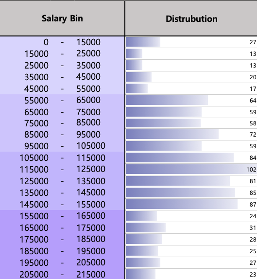
=IF(RAND()<0.2,RANDBETWEEN($Q$2,$S$6),IF(RAND()<0.5,RANDBETWEEN($Q$7,$S$11),IF(RAND()<0.5, RANDBETWEEN($Q$12,$S$16),IF(RAND()<0.2,RANDBETWEEN($Q$17,$S$22),RANDBETWEEN($Q$7,$S$16)))))- Chance of Coming Into the Store


=IFS(AND(A2>$Q$2,A2<$S$6),IF(RAND()<$U$2,"YES","NO"),AND(A2>$Q$7,A2<$S$11),IF(RAND()<$U$7,"YES","NO"), AND(A2>$Q$12,A2<$S$16),IF(RAND()<$U$12,"YES","NO"),AND(A2>$Q$17,A2<$S$22),IF(RAND()<$U$17,"YES","NO"))- Make a personalized decision (BUY or No) based on the in-store time
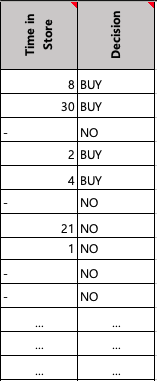
Customers entering the store will have a randomly assigned time spent in-store, ranging from 1 to 30 minutes.
The probability of making a purchase will vary based on the customer’s time spent in the store. Customers who spend more than 10 minutes in the store will have a 50% chance of making a purchase, those with less than 2 minutes will have a 10% chance, while others will have a 50% probability of deciding whether to buy or not.
=IF(B2="YES",RANDBETWEEN(1,30),"-")

=IF(C2="-","NO",IF(C2>10,IF(RAND()<0.5,"BUY","NO"),IF(C2<2,IF(RAND()<0.1,"YES","NO"),IF(RAND()>0.5,"BUY","NO"))))- Customer Decision Regarding Jewelry Purchase
Professor Jones has offered a simulation for customers’ decisions on purchasing jewelry, including probabilities for each variable. However, I have enhanced the simulation by incorporating real-world examples of individuals with salaries. While the probabilities remain constant, they now align with the customer’s salary information and apply exclusively to those who have decided to make a purchase.
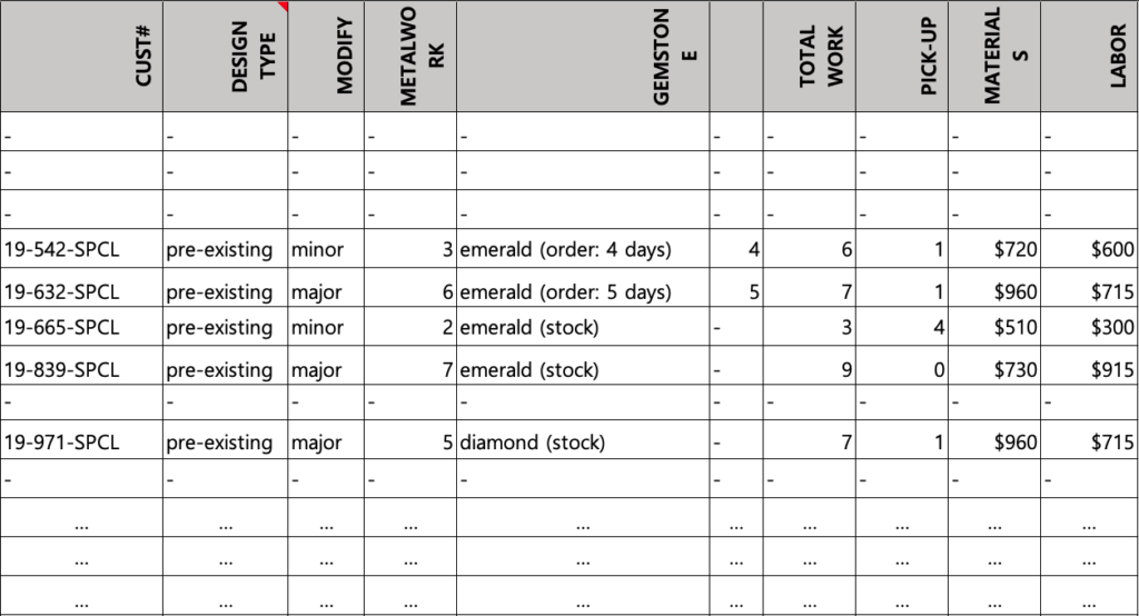
=IF(D3="BUY",IF(A3<$Q$12,IF(RAND()<0.7,"custom","pre-existing"),IF(RAND()<0.2,"custom","pre-existing")),"-")Final Simulation
Statistical Analysis
Original Data: Using the fixed statistics from one of the simulation and generating testing data.
Simulated Data: Using the active statistics from the simulation and generating testing data.
The Result in the Change of Parameters
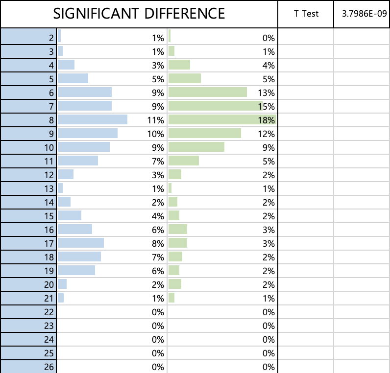
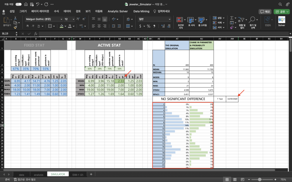
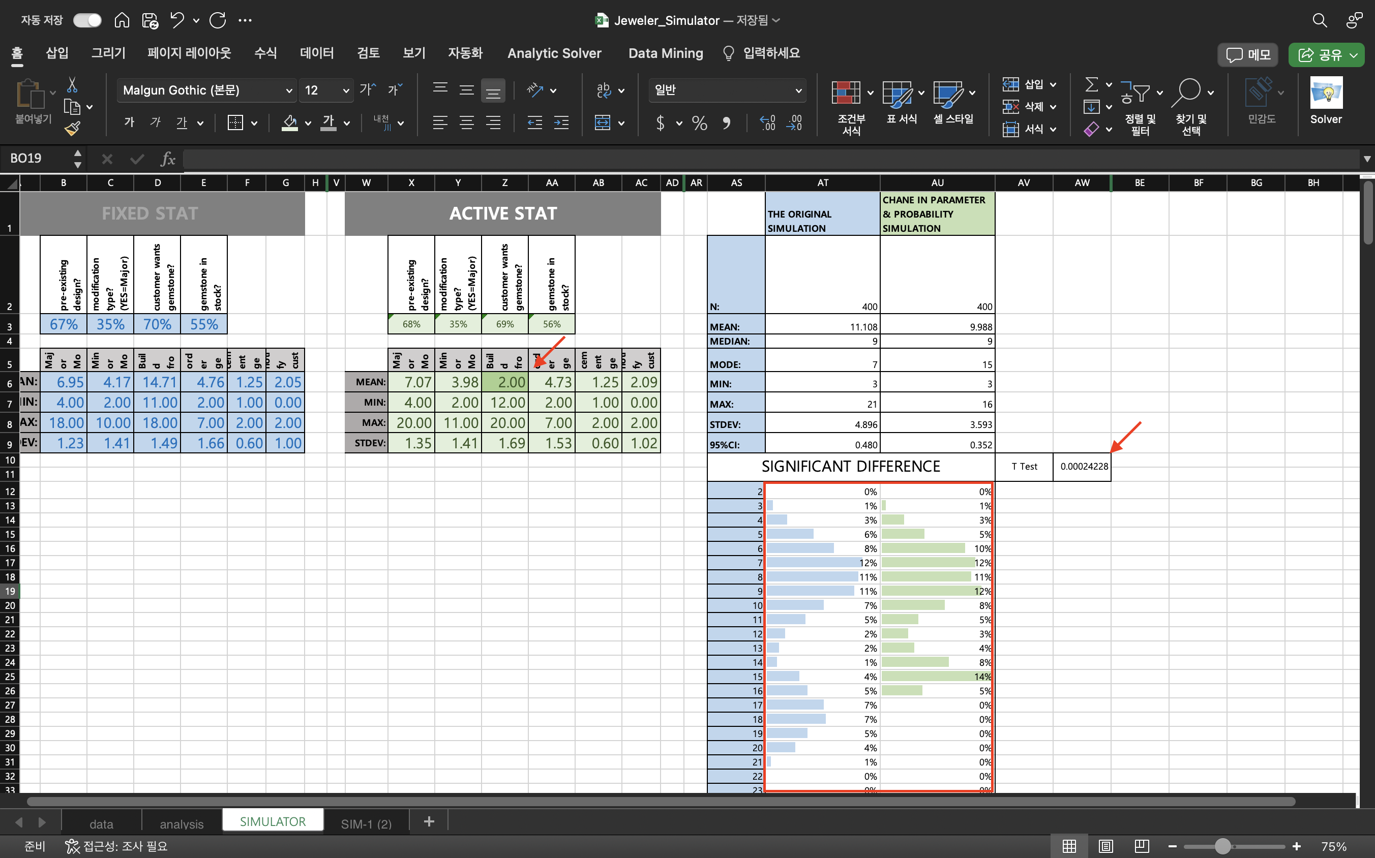
Scenario 1: If we were to purchase a new computer-controlled reductive-manufacturing platform capable to reducing the metal-working time to build a new custom piece by an average of two days and cutting the standard deviation in half, will it make a significant difference in the total time to produce our jewelry?
Observation:
By reducing the average day of wait for metal work 2 days, the entire graph shafted to the earlier days making it to have significant difference
November 2017 ~ December 2017
Statistics
Utilize simulations to conduct simple experiments that help in understanding the difference between statistics and reality and to grasp the true nature of statistics.
This project employs Excel-based simulations to introduce controlled variables and probabilities, effectively randomizing the original training data. Subsequently, simple statistics are extracted from the randomized data, providing the foundation for generating new testing data. The project then compares the original training data with the testing data, analyzing the impact of subtle manipulations in variables and probabilities on the outcomes.
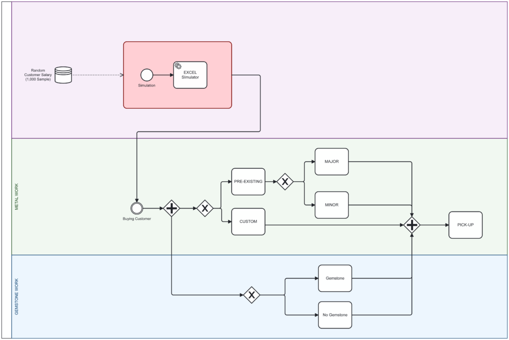
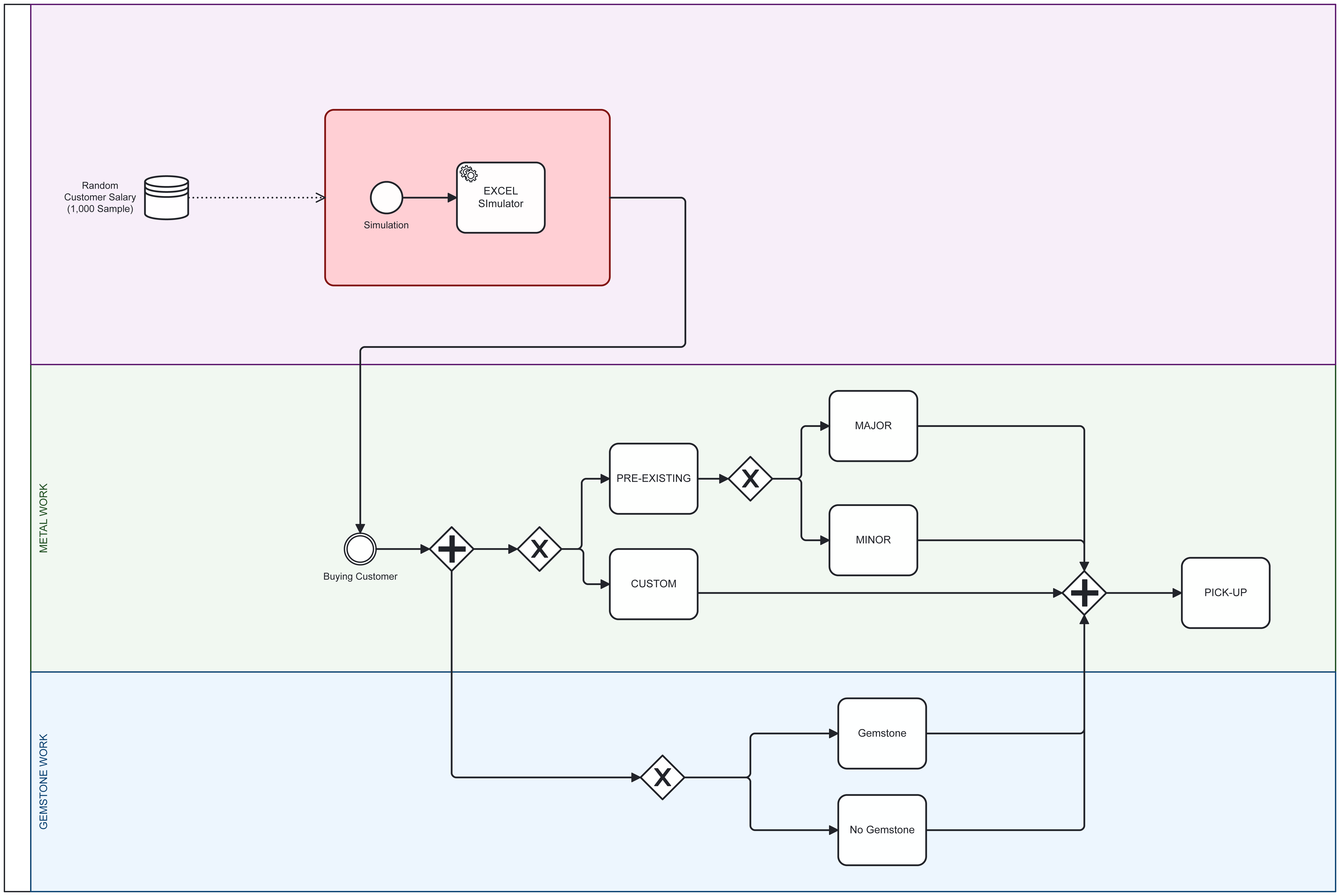
[Customer Decision Process in Jewelry Store (BPMN)]
Generate Testing Data Sample
With the goal of producing reasonable and realistic data during the simulation, I decided to introduce a few variables and limitations in the probabilities employed.
#1 Establish salary bins and restrict the distribution within each salary group.


=IF(RAND()<0.2,RANDBETWEEN($Q$2,$S$6),IF(RAND()<0.5,RANDBETWEEN($Q$7,$S$11),IF(RAND()<0.5, RANDBETWEEN($Q$12,$S$16),IF(RAND()<0.2,RANDBETWEEN($Q$17,$S$22),RANDBETWEEN($Q$7,$S$16)))))
#2 Chance of Coming Into the Store

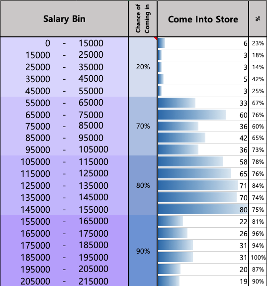
=IFS(AND(A2>$Q$2,A2<$S$6),IF(RAND()<$U$2,”YES”,”NO”),AND(A2>$Q$7,A2<$S$11),IF(RAND()<$U$7,”YES”,”NO”), AND(A2>$Q$12,A2<$S$16),IF(RAND()<$U$12,”YES”,”NO”),AND(A2>$Q$17,A2<$S$22),IF(RAND()<$U$17,”YES”,”NO”))
#3 Make a personalized decision (BUY or No) based on the in-store time
Customers entering the store will have a randomly assigned time spent in-store, ranging from 1 to 30 minutes.
The probability of making a purchase will vary based on the customer’s time spent in the store. Customers who spend more than 10 minutes in the store will have a 50% chance of making a purchase, those with less than 2 minutes will have a 10% chance, while others will have a 50% probability of deciding whether to buy or not.

=IF(B2=”YES”,RANDBETWEEN(1,30),”-“)
=IF(C2=”-“,”NO”,IF(C2>10,IF(RAND()<0.5,”BUY”,”NO”),IF(C2<2,IF(RAND()<0.1,”YES”,”NO”),IF(RAND()>0.5,”BUY”,”NO”))))
#4 Customer Decision Regarding Jewelry Purchase
Professor Jones has offered a simulation for customers’ decisions on purchasing jewelry, including probabilities for each variable. However, I have enhanced the simulation by incorporating real-world examples of individuals with salaries. While the probabilities remain constant, they now align with the customer’s salary information and apply exclusively to those who have decided to make a purchase.

=IF(D3=”BUY”,IF(A3<$Q$12,IF(RAND()<0.7,”custom”,”pre-existing”),IF(RAND()<0.2,”custom”,”pre-existing”)),”-“)
Final Simulation
Commencing from individual salary, the time taken in each jewelry process and the purchasing decision.
General Statistics Across Different Salary Ranges.
Statistical Analysis
Original Data: Using the fixed statistics from one of the simulation and generating testing data.
Simulated Data: Using the active statistics from the simulation and generating testing data.
The Result in the Change of Parameters
Scenario 1:
If we were to purchase a new computer-controlled reductive-manufacturing platform capable to reducing the metal-working time to build a new custom piece by an average of two days and cutting the standard deviation in half, will it make a significant difference in the total time to produce our jewelry?
Observation:
By reducing the average day of wait for metal work 2 days, the entire graph shafted to the earlier days making it to have significate differnce
Scenario 2:
If we were to hold more gemstones in inventory, reducing the need to order and wait by 50%, will this make a significant difference in the total time to produce our jewelry?
Observation:
By reducing the average day of wait for metal work 2 days, the entire graph shafted to the earlier days making it to have significant difference

Scenario 3:
If the probability of customer choosing custom or pre-existing design change, will it make significant difference? (customer with salary less than $105,000, now will have 10% chance to choose custom design)
Observation:
This change will influence customers’ decisions on design work, leading them to choose more pre-existing designs. From a logical standpoint, the availability of more pre-existing design choices reduces the customer wait time for their final product.
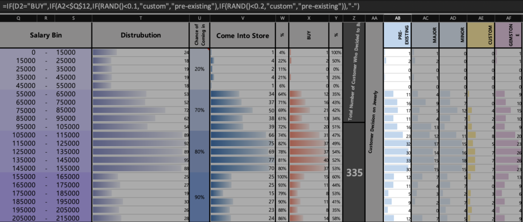
As a result, significant differences arise when the customer’s decision changes. Also, from the distribution graph, it is clear that the early wait time has increased, while the later wait time has reduced, indicating that more customers are now receiving their products faster.
